Comparison of six regridding algorithms

xESMF exposes five different regridding algorithms from the ESMF library:

• bilinear: ESMF.RegridMethod.BILINEAR

• conservative: ESMF.RegridMethod.CONSERVE

• conservative_normed: ESMF.RegridMethod.CONSERVE

• patch: ESMF.RegridMethod.PATCH

• nearest_s2d: ESMF.RegridMethod.NEAREST_STOD

• nearest_d2s: ESMF.RegridMethod.NEAREST_DTOS

where conservative_normed is just the conservative method with the normalization set to ESMF.NormType.FRACAREA instead of the default norm_type=ESMF.NormType.DSTAREA.

This notebook demonstrates how these algorithms behave in different situations.

Notes

• bilinear and conservative should be the most commonly used methods. They are both monotonic (i.e. will not create new maximum/minimum).

• Nearest neighbour methods, either source to destination (s2d) or destination to source (d2s), could be useful in special cases. Keep in mind that d2s is highly non-monotonic.

• Patch is ESMF’s unique method, producing highly smooth results but quite slow.

• From the ESMF documentation:

  The weight \(w_{ij}\) for a particular source cell \(i\) and destination cell \(j\) are calculated as \(w_{ij}=f_{ij} * A_{si}/A_{dj}\). In this equation \(f_{ij}\) is the fraction of the source cell \(i\) contributing to destination cell \(j\), and \(A_{si}\) and \(A_{dj}\) are the areas of the source and destination cells.

  For conservative_normed,

  … then the weights are further divided by the destination fraction. In other words, in that case \(w_{ij}=f_{ij} * A_{si}/(A_{dj}*D_j)\) where \(D_j\) is fraction of the destination cell that intersects the unmasked source grid.

Detailed explanations are available on ESMPy documentation.

Preparation

%matplotlib inline
import matplotlib.pyplot as plt
import cartopy.crs as ccrs
import numpy as np
import xarray as xr
import xesmf as xe

method_list = [
    "bilinear",
    "conservative",
    "conservative_normed",
    "nearest_s2d",
    "nearest_d2s",
    "patch",
]

ds_in = xe.util.grid_global(20, 15)  # input grid
ds_fine = xe.util.grid_global(4, 4)  # high-resolution target grid
ds_coarse = xe.util.grid_global(30, 20)  # low-resolution target grid

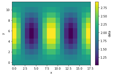
Make a wave field that is widely used in regridding benchmarks.

ds_in["data"] = xe.data.wave_smooth(ds_in["lon"], ds_in["lat"])
ds_in

<xarray.Dataset>
Dimensions:  (y: 12, x: 18, y_b: 13, x_b: 19)
Coordinates:
    lon      (y, x) float64 -170.0 -150.0 -130.0 -110.0 ... 130.0 150.0 170.0
    lat      (y, x) float64 -82.5 -82.5 -82.5 -82.5 ... 82.5 82.5 82.5 82.5
    lon_b    (y_b, x_b) int64 -180 -160 -140 -120 -100 ... 100 120 140 160 180
    lat_b    (y_b, x_b) int64 -90 -90 -90 -90 -90 -90 -90 ... 90 90 90 90 90 90
Dimensions without coordinates: y, x, y_b, x_b
Data variables:
    data     (y, x) float64 2.016 2.009 1.997 1.987 ... 1.987 1.997 2.009 2.016

ds_in["data"].plot()

<matplotlib.collections.QuadMesh at 0x7fcc27f6db80>

def regrid(ds_in, ds_out, dr_in, method):
    """Convenience function for one-time regridding"""
    regridder = xe.Regridder(ds_in, ds_out, method, periodic=True)
    dr_out = regridder(dr_in)
    return dr_out

When dealing with global grids, we need to set periodic=True, otherwise data along the meridian line will be missing.

Increasing resolution

for method in method_list:
    print(method)
    %time ds_fine[method] = regrid(ds_in, ds_fine, ds_in['data'], method)
    print('')

bilinear
CPU times: user 386 ms, sys: 24.9 ms, total: 410 ms
Wall time: 408 ms

conservative
CPU times: user 66.8 ms, sys: 3.79 ms, total: 70.6 ms
Wall time: 70.4 ms

conservative_normed
CPU times: user 84.6 ms, sys: 266 µs, total: 84.9 ms
Wall time: 84.6 ms

nearest_s2d
CPU times: user 29.6 ms, sys: 0 ns, total: 29.6 ms
Wall time: 29.4 ms

nearest_d2s
CPU times: user 8.44 ms, sys: 0 ns, total: 8.44 ms
Wall time: 8.22 ms

patch
CPU times: user 420 ms, sys: 12.3 ms, total: 432 ms
Wall time: 431 ms

Nearest neighbour algorithms are very fast while the patch method is quite slow.

fig, axes = plt.subplots(3, 2, figsize=[8, 8])

for i, method in enumerate(method_list):
    ax = axes.flatten()[i]
    ds_fine[method].plot.pcolormesh(ax=ax)
    ax.set_title(method, fontsize=15)

plt.tight_layout()

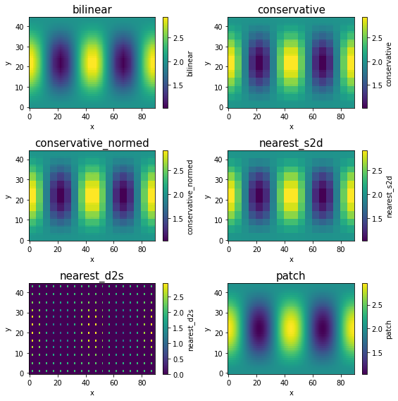
When regridding from low-resolution to high-resolution, bilinear and patch will produce smooth results, while conservative and nearest_s2d will preserve the original coarse grid structure (although the data is now defined on a finer grid.).

nearest_d2s is quite different from others: One source point can be mapped to only one destination point. Because we have far less source points (on a low-resolution grid) than destination points (on a high-resolution grid), most destination points cannot receive any data so they just have zero values. Only the destination points that are closest to source points can receive data.

Decreasing resolution

for method in method_list:
    ds_coarse[method] = regrid(ds_in, ds_coarse, ds_in["data"], method)

fig, axes = plt.subplots(3, 2, figsize=[8, 8])

for i, method in enumerate(method_list):
    ax = axes.flatten()[i]
    ds_coarse[method].plot.pcolormesh(ax=ax)
    ax.set_title(method, fontsize=15)
plt.tight_layout()

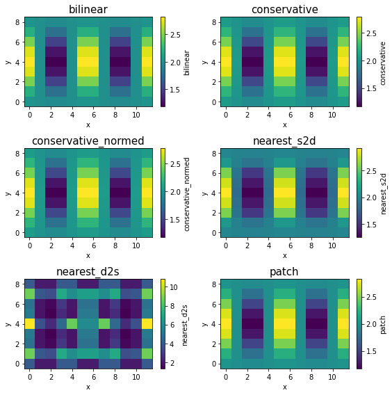
When regridding from high-resolution to low-resolution, all methods except nearest_d2s produce similar results here. But that’s largely because the input data is smooth. For real-world data, it is generally recommended to use conservative for decreasing the resolution, because it takes average over small source grid boxes, while bilinear and nearest_s2d effectively throw away most of source grid boxes.

nearest_d2s is again different: Every source point has to be mapped to a destination point. Because we have far more source points (on a high-resolution grid) than destination points (on a low-resolution grid), a single destination point will receive data from multiple source points, which can accumulate to a large value (notice the colorbar range).