Masking and extrapolation in xESMF
(contributed by Raphael Dussin, based on previous work from jhamman, RondeauG, trondkr and others)
By default, xESMF treats NaNs like regular values hence potentially resulting in missing values bleeding into the regridded field and creating insconsistencies in the resulting masked array. To overcome this issue, we can use explicit masking of the source and target grids.
[1]:
import xarray as xr
import xesmf
import numpy as np
[2]:
import warnings

warnings.filterwarnings("ignore")
Preparing the grids
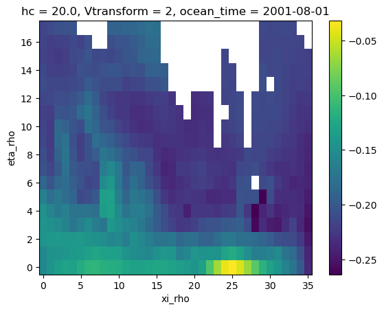
For this tutorial, we’re using a dataset from the ROMS ocean model from this xarray tutorial
[3]:
ds = xr.tutorial.open_dataset("ROMS_example.nc", chunks={"ocean_time": 1})
To use conservative regidding, we need the cells corners. Since they are not provided, we are creating some using a crude approximation. Please don’t try this at home!
[4]:
lon_centers = ds["lon_rho"].values
lat_centers = ds["lat_rho"].values

lon_corners = 0.25 * (
    lon_centers[:-1, :-1]
    + lon_centers[1:, :-1]
    + lon_centers[:-1, 1:]
    + lon_centers[1:, 1:]
)

lat_corners = 0.25 * (
    lat_centers[:-1, :-1]
    + lat_centers[1:, :-1]
    + lat_centers[:-1, 1:]
    + lat_centers[1:, 1:]
)

ds["lon_psi"] = xr.DataArray(data=lon_corners, dims=("eta_psi", "xi_psi"))
ds["lat_psi"] = xr.DataArray(data=lat_corners, dims=("eta_psi", "xi_psi"))

ds = ds.assign_coords({"lon_psi": ds["lon_psi"], "lat_psi": ds["lat_psi"]})

# remove exterior rho points and cut 9 extra points to make
# zeta divisible by 10 for coarsening
ds = ds.isel(
    eta_rho=slice(1, -10),
    xi_rho=slice(1, -10),
    eta_psi=slice(0, -9),
    xi_psi=slice(0, -9),
)
We also need a coarse resolution grid. We’re going to build one by coarsening the ROMS dataset. coarsen.mean() typically works as a nan-mean on the 10x10 blocks of the grid so the resulting land mask looks like a flooded version of the original.
[5]:
ds_coarse = xr.Dataset()

ds_coarse["zeta"] = xr.DataArray(
    ds["zeta"].coarsen(xi_rho=10, eta_rho=10).mean().values,
    dims=("ocean_time", "eta_rho", "xi_rho"),
)
# we want to subsample coordinates instead of coarsening them
ds_coarse["lon_rho"] = xr.DataArray(
    ds["lon_rho"].values[::10, ::10], dims=("eta_rho", "xi_rho")
)
ds_coarse["lon_psi"] = xr.DataArray(
    ds["lon_psi"].values[::10, ::10], dims=("eta_psi", "xi_psi")
)
ds_coarse["lat_rho"] = xr.DataArray(
    ds["lat_rho"].values[::10, ::10], dims=("eta_rho", "xi_rho")
)
ds_coarse["lat_psi"] = xr.DataArray(
    ds["lat_psi"].values[::10, ::10], dims=("eta_psi", "xi_psi")
)
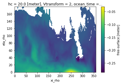
We now have our 2 grids to test the masking in xESMF. Now let’s say we want to conservatively remap the fine ocean model output onto the coarse resolution grid.
[6]:
ds["zeta"].isel(ocean_time=0).plot()
[6]:
<matplotlib.collections.QuadMesh at 0x150491d30>
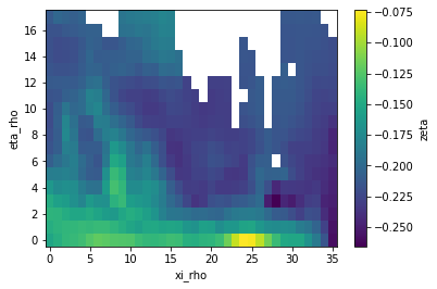
[7]:
ds_coarse["zeta"].isel(ocean_time=0).plot()
[7]:
<matplotlib.collections.QuadMesh at 0x1505c2990>
Regridding without a mask
As usual, xESMF expects fixed variable names for longitude/latitude in cell centers and corners:
[8]:
ds["lon"] = ds["lon_rho"]
ds["lat"] = ds["lat_rho"]
ds["lon_b"] = ds["lon_psi"]
ds["lat_b"] = ds["lat_psi"]

ds_coarse["lon"] = ds_coarse["lon_rho"]
ds_coarse["lat"] = ds_coarse["lat_rho"]
ds_coarse["lon_b"] = ds_coarse["lon_psi"]
ds_coarse["lat_b"] = ds_coarse["lat_psi"]
In our first test, there is no masking involved and we define the regridder the typical way:
[9]:
regrid_nomask = xesmf.Regridder(ds, ds_coarse, method="conservative")
[10]:
zeta_remapped = regrid_nomask(ds["zeta"])
[11]:
zeta_remapped.isel(ocean_time=0).plot()
[11]:
<matplotlib.collections.QuadMesh at 0x151d234d0>
Because of the missing values (NaNs) bleeding into the regridding, we end up with a land mask that is much bigger than the one of the coarse grid. That’s where masking is gonna help us getting it right.
Regridding with a mask
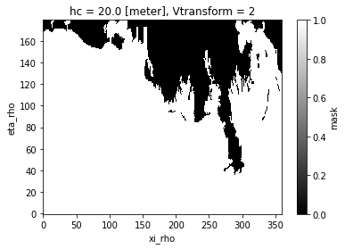
To use masking, we need to add a dataarray named mask to our datasets. Let’s define our masks on the high and coarse resolution grids from the missing values in the zeta array:
[12]:
ds["mask"] = xr.where(~np.isnan(ds["zeta"].isel(ocean_time=0)), 1, 0)
[13]:
ds["mask"].plot(cmap="binary_r")
[13]:
<matplotlib.collections.QuadMesh at 0x152dd1950>
[14]:
ds_coarse["mask"] = xr.where(
    ~np.isnan(ds_coarse["zeta"].isel(ocean_time=0)), 1, 0
)
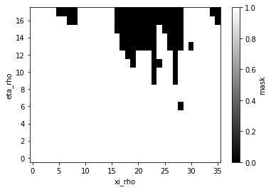
[15]:
ds_coarse["mask"].plot(cmap="binary_r")
[15]:
<matplotlib.collections.QuadMesh at 0x152edc050>
Now let’s try to regrid again:
[16]:
regrid_mask = xesmf.Regridder(ds, ds_coarse, method="conservative_normed")
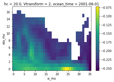
[17]:
zeta_remapped = regrid_mask(ds["zeta"])
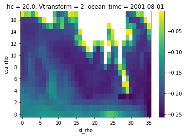
[18]:
zeta_remapped.isel(ocean_time=0).plot()
[18]:
<matplotlib.collections.QuadMesh at 0x152f8a990>

Now we have our conservative remapping consistent with the coarse grid, yay!!
Limitations and warnings
mask can only be 2D (ESMF design) so regridding a 3D field requires to generate regridding weights for each vertical level.
conservative method will give you a normalization by the total area of the target cell. Except for some specific cases, you probably want to use conservative_normed.
results with other methods (e.g. bilinear) may not give masks consistent with the coarse grid.
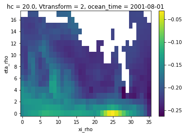
1. Conservative (un-normed) example
[19]:
regrid_masked2 = xesmf.Regridder(ds, ds_coarse, method="conservative")
zeta_remapped2 = regrid_masked2(ds["zeta"])
zeta_remapped2.isel(ocean_time=0).plot()
[19]:
<matplotlib.collections.QuadMesh at 0x1530f60d0>
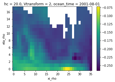
2. Bilinear example
[20]:
regrid_masked3 = xesmf.Regridder(ds, ds_coarse, method="bilinear")
zeta_remapped3 = regrid_masked3(ds["zeta"])
zeta_remapped3.isel(ocean_time=0).plot()
[20]:
<matplotlib.collections.QuadMesh at 0x15321c910>
Adaptive masking
The adaptive masking technique allows the reuse of weights for equal 2D fields that are only masked differently (eg. 3D fields with different land-sea masks / orography masks for each model layer or fields with masks varying over time). It is applicable for the conservative, patch and bilinear remapping methods and will either mask target cells or renormalize their resulting value, depending on how big of a fraction of the overlapping source grid cells is masked.
To use adaptive masking, the parameter skipna (and optionally also na_thres) has to be specified when applying the remapping weights, eg.:
ds_remapped = regridder(ds, [...] , skipna=True, na_thres=.25)
In case skipna is active, a given output point is set to NaN only if the ratio of missing values exceeds the threshold level set by na_thres, and else, a renormalization is conducted. For instance, when the center of a cell is computed linearly from its four corners, one of which is missing, the output value is set to NaN if na_thres is smaller than 0.25. Else, a renormalization is conducted.
na_thres can be any value in the interval [0., 1.] (the default being 1.), with na_thres = 0. meaning that adaptive masking will not have any effect. With the setting na_thres = 1., applying adaptive masking together with conservative weights is indistinguishable from applying conservative_normed weights (including a defined mask, as it has been shown in an example above).
[21]:
# Applying the 'conservative' weights without defined mask from an example above
#  with active adaptive masking and the default na_thres=1.
zeta_remapped = regrid_nomask(ds["zeta"], skipna=True)
zeta_remapped.isel(ocean_time=0).plot()
[21]:
<matplotlib.collections.QuadMesh at 0x1532d34d0>
Extrapolation
As we saw in the previous example, the bilinear interpolation was not providing a value at all the destination points. This is where the extrapolation becomes useful. xESMF allows to use the ESMF algorithms described in this section of the ESMF documentation. xESMF provides several extrapolation options to fill missing values outside the source domain:
nearest_s2d: assigns values from the nearest valid source cell.inverse_dist: computes a weighted average of nearby source cells using inverse-distance weighting.creep_fill: iteratively propagates values from valid cells into neighboring missing regions.
Please refer to the aforementioned documentation for more details.
[22]:
regrid_extrap_nearest_s2d = xesmf.Regridder(
    ds, ds_coarse, method="bilinear", extrap_method="nearest_s2d"
)
[23]:
zeta_remapped_extrap_nearest_s2d = regrid_extrap_nearest_s2d(ds["zeta"])
[24]:
zeta_remapped_extrap_nearest_s2d.isel(ocean_time=0).plot()
[24]:
<matplotlib.collections.QuadMesh at 0x15a21e990>
Unlike nearest-neighbor approaches, creep_fill produces smoother and more physically consistent fields because it propagates information gradually across neighboring cells instead of introducing sharp, pointwise jumps. When using creep_fill, a few constraints must be respected:
extrap_num_levelsmust be explicitly providedcreep_fillcannot be used together with conservative or conservative_normed regridding.
[25]:
regrid_extrap_creep_fill = xesmf.Regridder(
    ds,
    ds_coarse,
    method="bilinear",
    extrap_method="creep_fill",
    extrap_num_levels=10,
)
[26]:
zeta_remapped_extrap_creep_fill = regrid_extrap_creep_fill(ds["zeta"])
[27]:
zeta_remapped_extrap_creep_fill.isel(ocean_time=0).plot()
[27]:
<matplotlib.collections.QuadMesh at 0x15a379310>

Avoid extrapolation when remapping to a larger domain with the nearest_s2d method
When remapping to a larger domain with the nearest_s2d method, target grid cells outside the original source domain will get the value of the closest source grid cell at the domain edge, independent of the selected extrap_method. This can be an undesired behaviour. Please see Curvilinear Grid - Undesired Extrapolation for more details.