Use pure numpy array
Despite the “x” in its name (indicating xarray-compatible), xESMF can also work with basic numpy arrays. You don’t have to use xarray data structure if you don’t need to track metadata. As long as you have numpy arrays describing the input data and input/output coordinate values, you can perform regridding.
Code in this section is adapted from an xarray example.
[1]:
# not importing xarray here!
%matplotlib inline
import matplotlib.pyplot as plt
import numpy as np
import xesmf as xe
Rectilinear grid
Input data
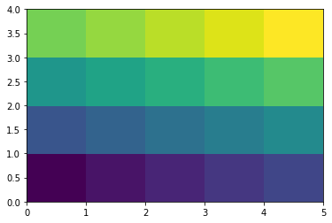
Just make some fake data.
[2]:
data = np.arange(20).reshape(4, 5)
plt.pcolormesh(data)
[2]:
<matplotlib.collections.QuadMesh at 0x7f8f5b75af40>
Define grids
In previous examples we use xarray DataSet as input/output grids. But you can also use a simple dictionary:
[3]:
grid_in = {"lon": np.linspace(0, 40, 5), "lat": np.linspace(0, 20, 4)}

# output grid has a larger coverage and finer resolution
grid_out = {"lon": np.linspace(-20, 60, 51), "lat": np.linspace(-10, 30, 41)}
Perform regridding
[4]:
regridder = xe.Regridder(grid_in, grid_out, "bilinear")
regridder
[4]:
xESMF Regridder
Regridding algorithm:       bilinear
Input grid shape:           (4, 5)
Output grid shape:          (41, 51)
Output grid dimension name: ('lat', 'lon')
Periodic in longitude?      False
The regridder here has no difference from the ones made from xarray DataSet. You can use it to regrid DataArray or just a basic numpy.ndarray:
[5]:
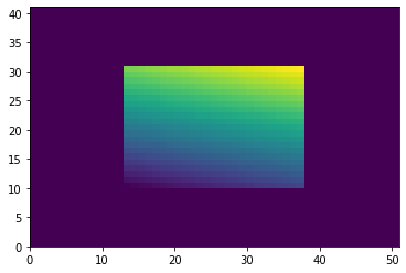
data_out = regridder(data)  # regrid a basic numpy array
data_out.shape
[5]:
(41, 51)
Check results
[6]:
plt.pcolormesh(data_out)
[6]:
<matplotlib.collections.QuadMesh at 0x7f8f5adc65e0>
Curvilinear grid
Grids
We use the previous input data, but now assume it is on a curvilinear grid described by 2D arrays. We also computed the cell corners, for two purposes:
Visualization with
plt.pcolormesh(using cell centers will miss one row&column)Conservative regridding with xESMF (corner information is required for conservative method)
[7]:
# cell centers
lon, lat = np.meshgrid(np.linspace(-20, 20, 5), np.linspace(0, 30, 4))
lon += lat / 3
lat += lon / 3

# cell corners
lon_b, lat_b = np.meshgrid(np.linspace(-25, 25, 6), np.linspace(-5, 35, 5))
lon_b += lat_b / 3
lat_b += lon_b / 3
[8]:
plt.pcolormesh(lon_b, lat_b, data)
plt.scatter(lon, lat)  # show cell center
plt.xlabel("lon")
plt.ylabel("lat")
[8]:
Text(0, 0.5, 'lat')

For the output grid, just use a simple rectilinear one:
[9]:
lon_out_b = np.linspace(-30, 40, 36)  # bounds
lon_out = 0.5 * (lon_out_b[1:] + lon_out_b[:-1])  # centers

lat_out_b = np.linspace(-20, 50, 36)
lat_out = 0.5 * (lat_out_b[1:] + lat_out_b[:-1])
To use conservative algorithm, both input and output grids should contain 4 variables: lon, lat, lon_b, lon_b.
[10]:
grid_in = {"lon": lon, "lat": lat, "lon_b": lon_b, "lat_b": lat_b}

grid_out = {
    "lon": lon_out,
    "lat": lat_out,
    "lon_b": lon_out_b,
    "lat_b": lat_out_b,
}
Regridding
[11]:
regridder = xe.Regridder(grid_in, grid_out, "conservative")
regridder
[11]:
xESMF Regridder
Regridding algorithm:       conservative
Input grid shape:           (4, 5)
Output grid shape:          (35, 35)
Output grid dimension name: ('lat', 'lon')
Periodic in longitude?      False
[12]:
data_out = regridder(data)
data_out.shape
[12]:
(35, 35)
Results
[13]:
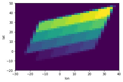
plt.pcolormesh(lon_out_b, lat_out_b, data_out)
plt.xlabel("lon")
plt.ylabel("lat")
[13]:
Text(0, 0.5, 'lat')
All possible combinations
All \(2 \times 2\times 2 = 8\) combinations would work:
Input grid:
xarray.DataSetordictOutput grid:
xarray.DataSetordictInput data:
xarray.DataArrayornumpy.ndarray
The output data type will be the same as input data.