Averaging over a region

Although this may not sound like real regridding, averaging a gridded field over a region is supported by ESMF. This works because the conservative regridding method preserves the areal average of the input field. That is, the value at each output grid cell is the average input value over the output grid area. Instead of mapping the input field unto rectangular outputs cells, it’s mapped unto an irregular mesh defined by an outer polygon. In other words, applying the regridding weights computes the exact areal-average of the input grid over each polygon.

This process relies on converting shapely.Polygon and shapely.MultiPolygon objects into ESMF.Mesh objects. However, ESMF meshes do not support all features that come with shapely’s (Multi)Polyons. Indeed, mesh elements do not support interior holes, or multiple non-touching parts, as do shapely objects. The xesmf.SpatialAverager class works around these issues by computing independent weights for interior holes and multi-part geometries, before combining the weights.

Transforming polygons into a ESMF.Mesh is a slow process. Users looking for faster (but approximate) methods may want to explore regionmask or clisops.

Also, note that low resolution polygons such as large boxes might get distorted when mapped on a sphere. Make sure polygon segments are at sufficiently high resolution, on the order of 1°. The shapely package (v2) has a `segmentize function <https://shapely.readthedocs.io/en/latest/reference/shapely.segmentize.html>`__ to add vertices to polygon segments.

The following example shows just how simple it is to compute the average over different countries. The notebook used geopandas, a simple and efficient container for geometries, and descartes for plotting maps. Make sure both packages are installed, as they are not xesmf dependencies.

[1]:

%matplotlib inline
import matplotlib.pyplot as plt
import geopandas as gpd
import pandas as pd
from shapely.geometry import Polygon, MultiPolygon
import numpy as np
import xarray as xr
import xesmf as xe
import warnings

warnings.filterwarnings("ignore")
xr.set_options(display_style='text')

[1]:

<xarray.core.options.set_options at 0x7fdc3c03b1c0>

Simple example

In this example we’ll create a synthetic global field, then compute its average over six countries.

Download country outlines

[2]:

# Load some polygons from the internet
regs = gpd.read_file(
    "https://cdn.jsdelivr.net/npm/world-atlas@2/countries-10m.json"
)

# Select a few countries for the sake of the example
regs = regs.iloc[[5, 9, 37, 67, 98, 155]]

# Simplify the geometries to a 0.02 deg tolerance, which is 1/100 of our grid.
# The simpler the polygons, the faster the averaging, but we lose some precision.
regs["geometry"] = regs.simplify(tolerance=0.02, preserve_topology=True)
regs

[2]:

	id	name	geometry
5	032	Argentina	MULTIPOLYGON (((-67.19287 -22.82225, -67.02727...
9	156	China	MULTIPOLYGON (((77.79858 35.49614, 77.66178 35...
37	710	South Africa	MULTIPOLYGON (((19.98200 -24.75230, 20.10800 -...
67	724	Spain	MULTIPOLYGON (((-5.34065 35.84736, -5.37665 35...
98	466	Mali	POLYGON ((-12.26352 14.77561, -12.13752 14.784...
155	484	Mexico	MULTIPOLYGON (((-97.13797 25.96581, -97.16677 ...

[3]:

# Create synthetic global data
ds = xe.util.grid_global(2, 2)
ds = ds.assign(field=xe.data.wave_smooth(ds.lon, ds.lat))
ds

[3]:

<xarray.Dataset>
Dimensions:  (x: 180, x_b: 181, y: 90, y_b: 91)
Coordinates:
    lon      (y, x) float64 -179.0 -177.0 -175.0 -173.0 ... 175.0 177.0 179.0
    lat      (y, x) float64 -89.0 -89.0 -89.0 -89.0 ... 89.0 89.0 89.0 89.0
    lon_b    (y_b, x_b) int64 -180 -178 -176 -174 -172 ... 172 174 176 178 180
    lat_b    (y_b, x_b) int64 -90 -90 -90 -90 -90 -90 -90 ... 90 90 90 90 90 90
Dimensions without coordinates: x, x_b, y, y_b
Data variables:
    field    (y, x) float64 2.0 2.0 2.0 2.0 2.0 2.0 ... 2.0 2.0 2.0 2.0 2.0 2.0

[4]:

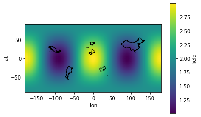
# Display the global field and countries' outline.
fig, ax = plt.subplots()
ds.field.plot(ax=ax, x="lon", y="lat")
regs.plot(ax=ax, edgecolor="k", facecolor="none")

[4]:

<AxesSubplot:xlabel='lon', ylabel='lat'>

../_images/notebooks_Spatial_Averaging_5_1.png

Compute the field average over each country

xesmf.SpatialAverager is a class designed to average an xarray.DataArray over a list of polygons. It behaves similarly to xesmf.Regridder, but has options to deal specifically with polygon outputs. It uses the conservative regridding, and can store and reuse weights.

[5]:

savg = xe.SpatialAverager(ds, regs.geometry, geom_dim_name="country")
savg

[5]:

xESMF SpatialAverager
Weight filename:            spatialavg_90x180_6.nc
Reuse pre-computed weights? False
Input grid shape:           (90, 180)
Output list length:         6

When called, the SpatialAverager instance returns a DataArray of averages over the geom dimension, here countries. lon and lat coordinates are the centroids each polygon.

[6]:

out = savg(ds.field)
out = out.assign_coords(country=xr.DataArray(regs["name"], dims=("country",)))
out

[6]:

<xarray.DataArray 'field' (country: 6)>
array([1.58448717, 1.49195654, 2.48197742, 2.5740491 , 2.89305772,
       1.26271837])
Coordinates:
    lon      (country) float64 -65.18 103.8 25.09 -3.646 -3.541 -102.5
    lat      (country) float64 -35.39 36.56 -29.0 40.23 17.35 23.95
  * country  (country) object 'Argentina' 'China' ... 'Mali' 'Mexico'
Attributes:
    regrid_method:  conservative

As the order of the polygons is conserved in the output, we can easily include the results back into our geopandas dataframe.

[7]:

regs["field_avg"] = out.values
regs

[7]:

	id	name	geometry	field_avg
5	032	Argentina	MULTIPOLYGON (((-67.19287 -22.82225, -67.02727...	1.584487
9	156	China	MULTIPOLYGON (((77.79858 35.49614, 77.66178 35...	1.491957
37	710	South Africa	MULTIPOLYGON (((19.98200 -24.75230, 20.10800 -...	2.481977
67	724	Spain	MULTIPOLYGON (((-5.34065 35.84736, -5.37665 35...	2.574049
98	466	Mali	POLYGON ((-12.26352 14.77561, -12.13752 14.784...	2.893058
155	484	Mexico	MULTIPOLYGON (((-97.13797 25.96581, -97.16677 ...	1.262718

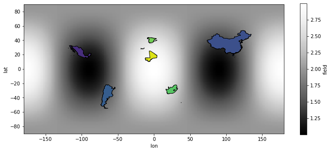
[8]:

fig, ax = plt.subplots(figsize=(12, 5))
ds.field.plot(ax=ax, x="lon", y="lat", cmap="Greys_r")
handles = regs.plot(
    column="field_avg", ax=ax, edgecolor="k", vmin=1, vmax=3, cmap="viridis"
)

../_images/notebooks_Spatial_Averaging_12_0.png

Extract the weight mask from the averager

The weights are stored in a sparse matrix structure in SpatialAverager.weights. The sparse matrix can be converted to a full DataArray, but note that this will increase memory usage proportional to the number of polygons.

[9]:

# Convert sparse matrix to numpy array, it has size : (n_in, n_out)
# So reshape to the same shape as ds + polygons
w = xr.DataArray(
    savg.weights.toarray().reshape(regs.geometry.size, *ds.lon.shape),
    dims=("country", *ds.lon.dims),
    coords=dict(country=out.country, **ds.lon.coords),
)
plt.subplots_adjust(top=0.9)
facets = w.plot(col="country", col_wrap=2, aspect=2, vmin=0, vmax=0.05)
facets.cbar.set_label("Averaging weights")

<Figure size 432x288 with 0 Axes>

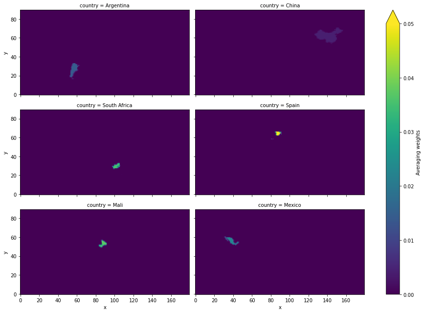
../_images/notebooks_Spatial_Averaging_14_1.png

This also allows to quickly check that the weights are indeed normalized, that the sum of each mask is 1.

[10]:

w.sum(dim=["y", "x"]).values

[10]:

array([1., 1., 1., 1., 1., 1.])